Meditative Marble (Bigmode Jam 23)
Roll a marble through a grassy landscape. A simulation of ball physics in a procedurally generating continuous world. I used this project to learn about on the fly 3D model generation, accurate 3D collisions, seamless swapping of models, 3rd person cameras, and noise functions.
Made in two weeks for bigmode game jam 2023.
-
Check out the Source Code
-
Download a build
This game was made using my
graphics rendering library.
I saw a trailer for a game called Exo One a while ago and the concept stuck in my head, so I’ve always wanted to try to implement ball physics in a wide open world to roll around. As this was a longer game jam, I thought it was the perfect opportunity to explore the kinds of maths involved and try and come up with my own solutions.
First, a high level description of the game before I dive into the technical details.
The game describes the map with a function of the form f(x, y) = z.
Using this function I generate a 3D mesh based on the player’s position and load it while they are playing. Once the mesh is loaded I swap the current one for the new one so the player sees the world as one continous mesh without noticing the swap.
For the world’s shape I use simplex noise of various resolutions combined to create the rolling hills with mountains effect.
The marble has acceleration, velocity, position and spin to create the illusion of a real ball. The player can add directional acceleration to the ball based on the camera’s view. The camera follows the player without clipping through the map, pulling back when the player speeds up and pointing in the direction the player moves.
Below are the details of the above overview.
3rd Person Camera
Link to the code file that this section discusses
The first part of this project I worked on was the third person camera. The goal is a camera that keeps a subject in frame and can rotate around it to view it from various angles. First I will describe the view matrix in general, then I will apply this to a 3rd person camera.
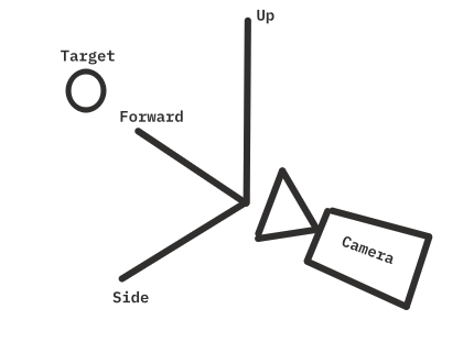
We can define a camera’s view matrix using a set of basis vectors (axes). We need a vector pointing towards the target (F), a vector pointing up (U), and one pointing to the side (S). We also need a camera’s position (P) in the world.
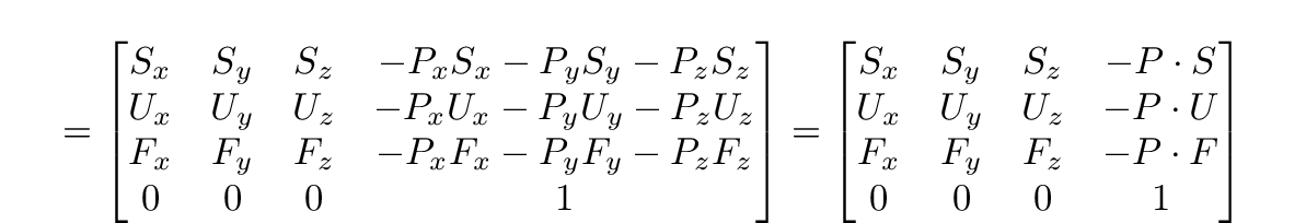
Our goal is a matrix which transforms a vector from it’s position in the world, to it’s position in relation to the camera. This is a change of basis (we want a vector in terms of the camera’s axes), which can be represented by matrix multiplication with the new basis vectors as the rows of a 3x3 matrix, which we expand to 4x4 so that we can translate the view by the position of the camera. The translation ensures moving the position of camera without it’s basis chaning will move a vertex in relation to the camera. This kind of matrix is called a view matrix, and it is the result of the following calculation.

Note that we can simplify this to a single matrix, as the transform matrix on the right of the multiplication will only affect the last column of the view matrix. Each entry in the last column is given by the dot product of the position (P) and each basis vector along that row. If we do the full matrix multiplication, the result is clear.
Now that we know how to represent a camera’s state in 3D, we have to restrict the axes and positions to be consistently pointing towards a moving target as we rotate around it. To make this simpler I store the camera’s position as a unit vector from the origin (I will call this local space) and only consider the target’s position when I build the view matrix.
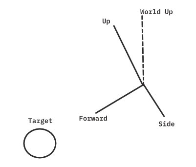
By considering a sphere around a target and a single point on the sphere’s surface, we can treat that point as the position of a camera that points towards the centre of the sphere to look at the target.
We start with a position representing a point on the sphere’s surface in local space, so the centre being observed is at position (0, 0, 0), as well as a radius for how far away from the target the camera should be. We also need a world up direction, this is because a third person camera doesn’t have any roll, it is always horizontal to the world, so we must have a consistent up facing direction (this is an arbitrary choice, but should probably be one of the world space’s basis vectors e.g (0, 0, 1)). We can now calculate the camera’s basis vectors.
Forward is just our position vector, as the target is at (0, 0, 0). We can then get a side-facing vector by doing the cross product of the world up vector and our target vector. Recall that the cross product gives a new vector perpendicular to the other two, but becauase world up and forward will usually not themselves be perpendicular, we need to normalize the side vector to ensure it has unit length. If this isn’t done, the camera would look like it was getting further away as the camera neared the top or bottom of the sphere. We can then recalculate our ideal perpendicular up vector with the cross product of the forward and side vectors. This gives us our three basis vectors for view space.
Finally we use the position of the target to get the last column’s values. The position of the camera is our position in local space times a distance value plus the position of the target. The distance value allows us to change the size of the sphere the camera is on. Putting it all together, the final view matrix can be built with the following code.
    forward = localpos;
    vec3 worldpos = localpos * radius + target;
    left = normalize(cross(worldUp, forward));
    up = cross(forward, left);

    view = mat4(1); //start with 4x4 identity matrix
    view[0][0] = left.x;
    view[1][0] = left.y;
    view[2][0] = left.z;
    view[3][0] = -dot(left, worldpos);
    view[0][1] = up.x;
    view[1][1] = up.y;
    view[2][1] = up.z;
    view[3][1] = -dot(up, worldpos);
    view[0][2] = forward.x;
    view[1][2] = forward.y;
    view[2][2] = forward.z;
    view[3][2] = -dot(forward, worldpos);
Now the only thing left is moving the camera around the sphere. With a third person camera one usually uses the input to manipulate it’s position around a subject. This means we need to track 2d input to 3d rotations around the sphere’s surface. As we have a fixed world up direction (ie no roll) we can simply track Y input to up and down motion and X input to sideways motion on the sphere.
Up and down motion is exactly rotation around the camera’s side axis, side-to-side motion is rotation around the up axis. Quaternions can be built using a rotation axis and an angle, then we can conjugate our camera’s position with that quaternion to rotate it around the sphere. For a given frame we get a 2D vector for the input direction, build a quaternion that encompasses rotation around the two axes by the input amount, then update the camera’s position using the quaternion.
quat qx = quat( cos(input.x), sin(input.x) * up);
quat qy = quat( cos(input.y), sin(input.y) * left);
quat q = qx * qy;
pos = q * pos * conjugate(q);
Note that at extreme angles, when the camera is at the very top or bottom of the sphere, the cross product of forward and world up will be 0, which cannot be normalized, leading to some jittery behaviour. This means we must limit our angle to some cutoff value at the extremes. I do this before I update the position.
float updot = dot(forward, worldUp); // == 1 if parallel, as these are unit vectors
// if above lim and moving up, or below -lim and moving down, don't move that way
if(updot > lim && input.y < 0 || -updot > lim && input.y > 0)
	input.y = 0;
Generating 3D Models With Code
Link to the code file that this section discusses
I wanted to learn about generating meshes with code so my goal was to take an arbitrary surface function and use it to generate a 3d model I could display in the game.
A surface in 3D is a two dimensional “part” of the space. So we can describe a surface using two parameters. Give a value for each parameter we can output a point in 3d space. By moving through the two parameters we can draw a surface (a graph of this function). If we use a continous (ie no breaks) function we can go through a range of inputs for the two parameters and get out a continous surface in 3D space. This is what I do to generate a mesh for a given function.
The mesh generation code can take any function of the form f(float, float) = vec3, as well as the starting and ending points of the two inputs, and a step value for how detailed the mesh should be.

Small Step Values

Large Step Values
You can also specify the uv density, which is how big or small a texture applied to the surface will look. There is an option to use smooth shading or not. With smooth shading off, vertices at the edges of triangles are not shared between neighbouring triangles. This give a visible polygon look.

Smooth Shading

No Smooth Shading
The structure of the mesh and how it is generated is illustrated well with the image that does not use smooth shading. I generate the meshes in a gridlike manner, for each step of each parameter there is a seperate square, which is made of two triangles. With smooth shading there is only one new vertex for each new square 90% of the time, as the other 3 vertices are shared with the neighbouring squares.
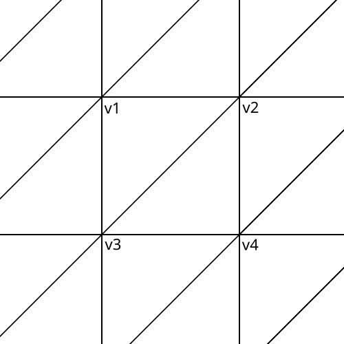
To generate a given square of the surface of the function, we determine the 4 verts by either making new ones, or using preexisting ones. To make a vertex we run the surface function on the values of the parameters for that corner, then we assign the vertex position that function’s return value. So the square has corners given by f(a, b), f(a + step_a, b), f(a, b + step_b), f(a + step_a, b + step_b) for our surface function f. Then the normal for that vertex is given by the average of the normals of the triangles that that vertex is shared between.
With all of the vertices build, the last thing to do is fill the index buffer with the indices of the square’s vertices. We need 6 indices to fully describe the two triangles making up the square. The only thing to be careful of is to be consistent with the winding order of the verts, as on most renderers only one side of a mesh is actually drawn. In this case I go with (3, 2, 1, 2, 3, 4) so that each triangle has the same winding order (anticlockwise). The user supplied surface function can always change the direction the mesh is generated in to turn a given surface inside out.
Now we have a vertex and index array that estimates the surface function within a range, giving us a mesh to draw. With the explaination finished, here are some examples of shapes generated by this technique.
genSurface([](float a, float b){
  float rad = 5;
  return glm::vec3(
    rad*sin(a)*cos(b),
    rad*sin(a)*sin(b),
    rad*cos(a));
}, true, 10.0f,
{0.0f, 3.1415 /* PI  */, 0.1f},
{0.0f, 6.283f /* 2PI */, 0.1f});

genSurface([](float a, float b){
  return glm::vec3(
    0.5*a*cos(b),
    0.5*a*sin(b),
    -a);
}, true, 10.0f,
{0.0f, 3.1415 /* PI  */, 0.1f},
{0.0f, 10.0f, 0.1f});

genSurface([](float x, float y){
  return glm::vec3(x, y, sin(x)*cos(y));
}, true, 10.0f,
{0.0f, 10.0f, 0.4f},
{0.0f, 10.0f, 0.4f});

genSurface([](float x, float y){
  float i[] = {x*0.5f, y*0.5f, 1.0f};
  return glm::vec3(x, y,
    noise::simplex<3>(i));
}, true, 10.0f,
{0.0f, 10.0f, 0.1f},
{0.0f, 10.0f, 0.1f});

Noise Functions
Link to the code file that this section discusses
I wanted to use this game as an opportunity to explore methods of procedural generation. After I got the mesh generation part working, I wanted to generate a map for the world. To make collision easier, the function to generate the map should take in an x and y coordinate and output a z coordinate for the height at that point. The drawback is that there can be no caves or overhanging terrain, but I think this simplification makes the code easier.
I decided to go with simplex noise to generate the height at each point. The final map uses multiple calls to a 3D simplex noise function added together. The first two inputs are the x and y coordinates for that point, and the third input is a random value that is fixed for the runtime of the program. This means there is a unique map each time the game is run.
Simplex noise is a smooth noise generating algorithm designed by ken perlin, which is an improvement on perlin noise that works with any number of dimensions. Here is the original description, and my main resource for this implementation. There are a few open source implementations, but I felt wrong to use this code without having any understanding for how it worked. As well as this, the implementations I could find had a unique function with different code for each dimension, for the sake of efficiency. I wanted to have function that would work for any arbitrary number of dimensions. The implementation I referenced the most is one for 1-4 dimensions by Stefan Gustavon, found here. I also used a hash array found here, by Ken Perlin. This is an array of 256 randomly distributed ints for use when generating the final random output.
The explainations below will omit the skewing and unskewing steps for finding the correct hypercube the input lies in and obtaining the unskewed simplex verticies.
Simplifed 2D Simplex Noise Explaination
Consider a grid of squares with whole number coordinates for each vertex. Our two inputs x, y define a point in this space.
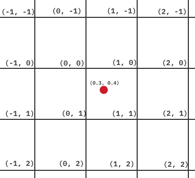
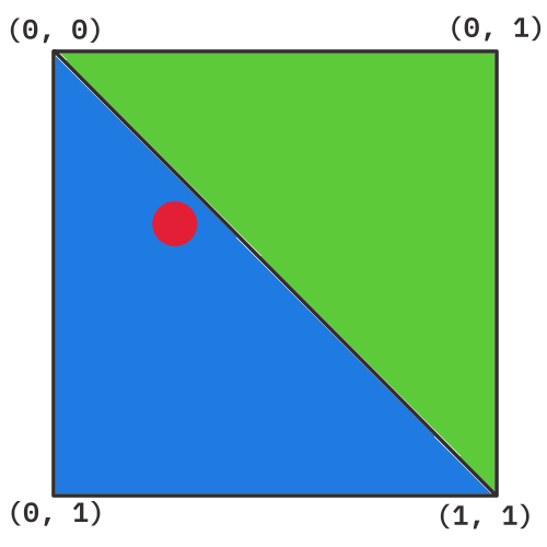
We then look at the grid square that the point falls into. If we start at the vertex on the top right, we can reach the bottom left corner by travelling through one other vertex (either (1, 0) or (0, 1)). These two paths each represent a different triangle. We then choose the triangle that our scaled point is lying in.
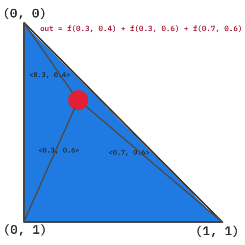
We then calculate the distance between our point and each of the vertices of the triangle. We input the resulting distances into a function with some pseudo-randomness and outputting a new number. Adding up all these outputs with some factor gives the final result of the noise function.
In N-Dimensions
Try to keep the 2D example in mind and consider what this means in 3D as we go over simplex noise with an arbitrary number of dimensions. We take our space and partition it into a grid (honeycomb) of hypercubes (n-dimensional squares) with integer vertices. We take n reals as input (x1, x2, ..., xn) and work out which hypercube it lies in. A simplex is an n-dimensional triangle, and we can partition a hypercube into distinct simplices (more details). We want to get the simplex that our input lies in, say our input is in hypercube with smallest coordinate (i1, i2, i3, ..., in). We consider a hypercube at the origin with vertex v1 = (0, 0, ..., 0). We sort our input by size, for example [x3, x2, xn, ..., x1], then we can get the vertices of the simplex by taking the next smallest of our inputs and adding 1 to the coordinate it corresponds to. Our input ordering would give v2 = (0, 0, 1, ..., 0) (as x3 was the smallest coord), v3 = (0, 1, 1, ..., 0) (x2 next smallest), v4 = (0, 1, 1, ..., 1) (xn next smallest), and so on until we get the last one which must be all 1s, vn+1 = (1, 1, 1, ..., 1). These vertices are then guarenteed to be for the simplex our point lies in within the hypercube. Finally for each simplex vertex we calculate the vector from the vertex to our input, for example for v3 we get d3 = <x1 - i1 + 0, x2 - i2 + 1, x3 - i3 + 1, ..., xn - in + 0>. We then take some randomness function (ie f) and input this vector o3 = f(d3). The final result is given by out = o1 + o2 + o3 + .. + on
Collisions with Surface Functions
In the code below we approximate the closest point on a surface given a point in 3d space.
struct fnArgs {float a; float b; };

/// Approximates local minimum of f
fnArgs localMinimum(float a, float b, std::function<float (float, float)> f) {
    float h = 0.1f; // small change in input to f
    float step = 0.1f; // step toward local minimum
    const int ITERS = 10; // how many steps to take
    for(int i = 0; i < ITERS; i++) {
		// approximate del(f(a, b))
		float ap = f(a + h, b); // positive change in f
		float bp = f(a, b + h);
		float an = f(a - h, b); // negative change in f
		float bn = f(a, b - h);
		// gradient in a, b direction
		float da = (ap - an)/(2*h); // divided by size of change
		float db = (bp - bn)/(2*h);
		// update a, b by a step in direction of least gradient
		a -= step*da;
		b -= step*db;
    }
    return {a, b};
}

/// Approximates nearest point to pos on fn
glm::vec3 nearestPoint(glm::vec3 pos, std::function<glm::vec3 (float, float)> fn) {
    // dist between our input pos and the surface pos squared
    std::function<float (float, float)> d2 = [&pos, &fn](float a, float b) {
		glm::vec3 d = pos - fn(a, b);
		return glm::dot(d, d);
    };
	// inital guess of closest point is point corresponding to a = x, b = y
    fnArgs g = localMinimum(pos.x, pos.y, d2);
    return fn(g.a, g.b);
}
Loading the World as the Player Moves
link to the code that this section discusses
TODO