Extending my complex function animation library to work with graphing functions of the form f(x, y) = g(x, y)

This is a continuation of my previous project where I outputted complex functions as images and animations, see the post here.

My goal is to be able to draw the graphs of functions and animate them using the functionality developed previously.

Here is a link to the source code for this project. There you can find more images and animations, as well as the code used to generate them.

Building the Functionality

The library’s image generating function calls a function for each pixel, which returns a colour. We can specify a pixel function that will generate our graph.

To begin I tried manually graphing x squared.

The graph line is quite hazy, but otherwise it is clearly x squared. The code to generate something like this is shown below. To graph f(x), we just need to get abs(f(x) - y) and scale it by some value, then use that as an intensity for a grayscale image. This gives a number closer to zero the closer that pixel is to the ideal graph line.

(canim:make-im 
 "build/x-squared.png" 
 300 300 
 (canim:make-pos :x -1 :y -1 :scale 2)
 :pixel-fn 
 (lambda (x y scale)
   (let* 
       ((intensity
	 (* 100 (abs (- (expt x 2) y))))
        (colour
	 (min (floor (* intensity 255)) 255)))
     (canim:make-colour
      colour colour colour 255))))

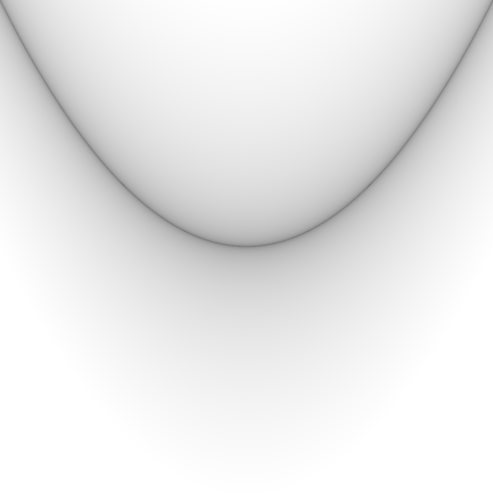
With a little fiddling, making a better use of cutoffs and scaling, we can have a much sharper line.

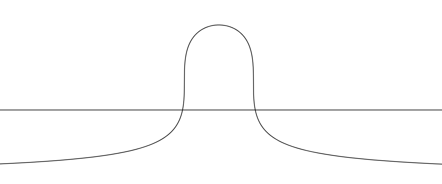
But already you can see an issue with having a fixed scaling/cutoff for each pixel. as x squared gets bigger, the line thins out. This happens because the cutoff, which determines the line thickness, is the same no matter the behaviour of the function in that area. Here is an explaination of why this occurs.

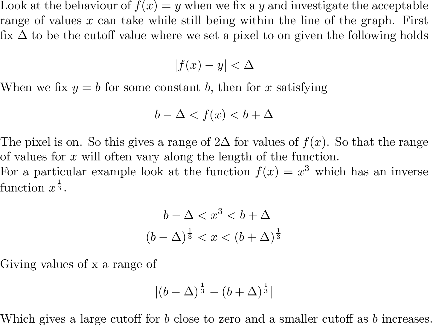
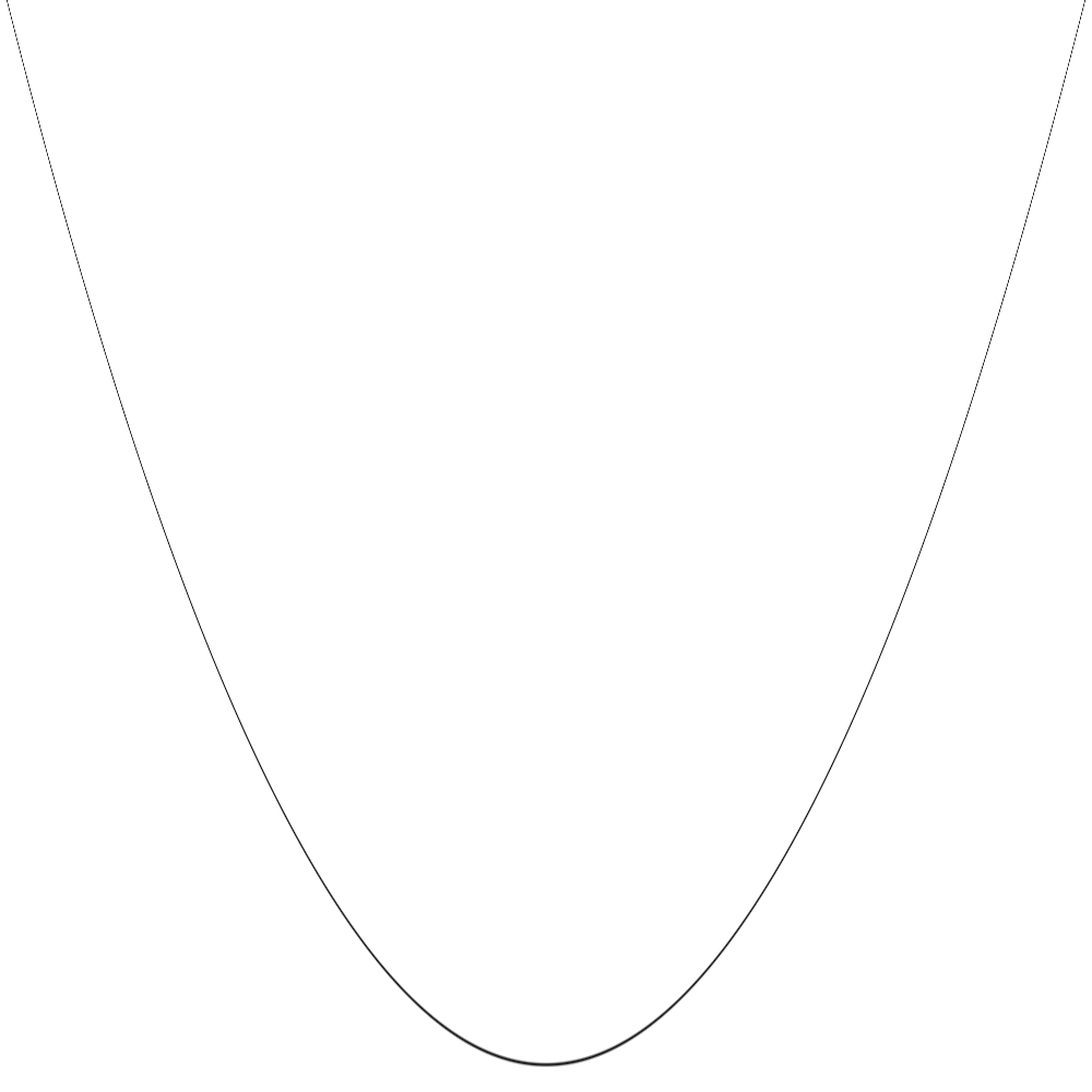
This is the graph of the cutoff value for x cubed with different values for y. The straight line is the value for the cutoff, the curvy line is the actual range that x gets.

f(x, y) = c

The next type of graphs I tried to draw were of the form f(x, y) = c for some constant c. Below we see the equation of a circle.

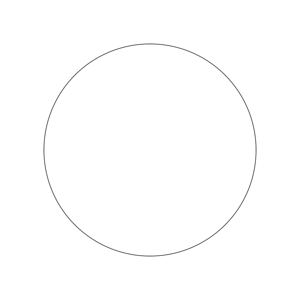
The distance to the point is determined using abs(f(x, y) - c).

I added the ability to send a list of functions to be drawn, so they are overlaid ontop of each other. Here we see circles of different radii.

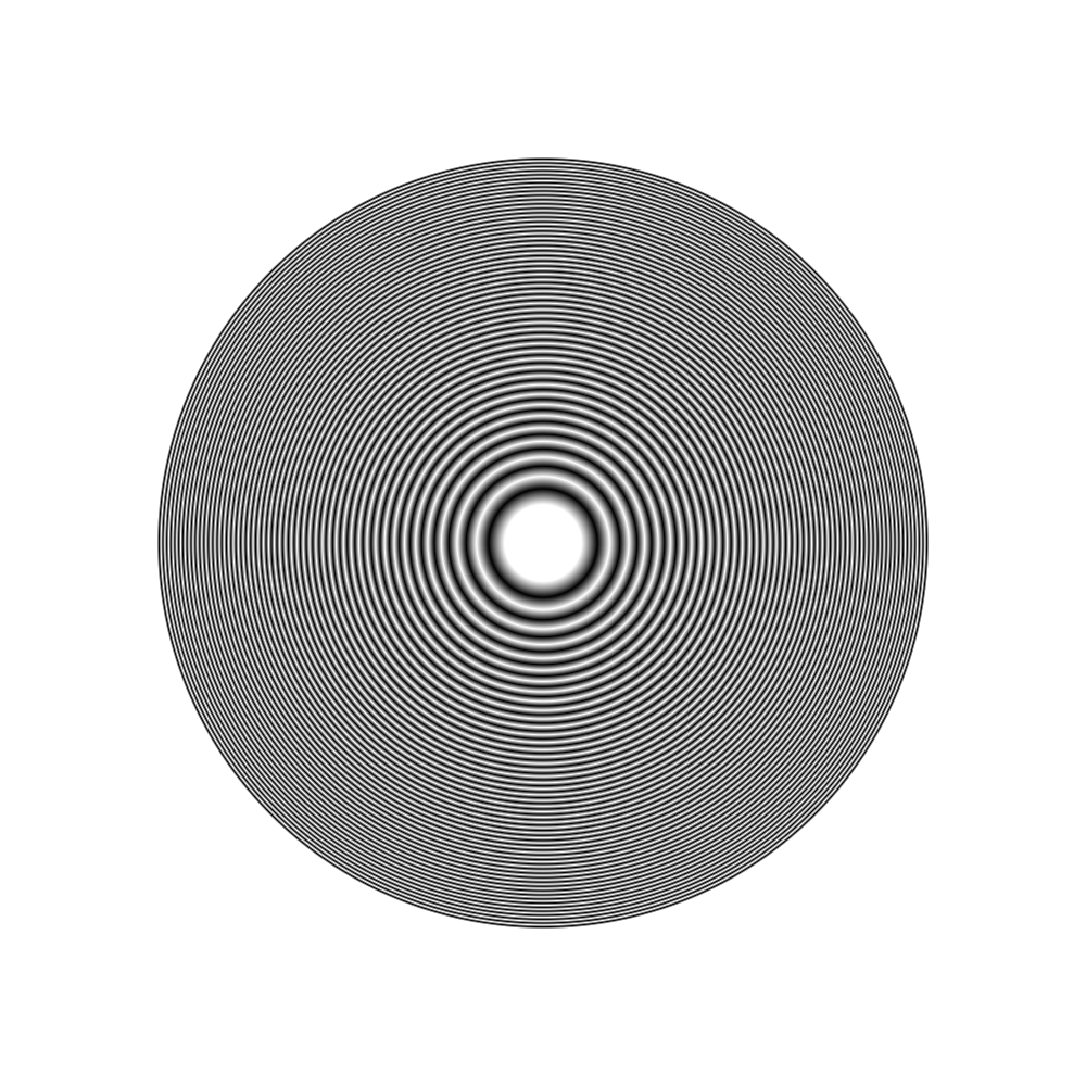
Initially it looked as if the circle’s thickness worked well, but, as with the 2nd x squared image, we see how the thickness of the line changes as we use different values for the radius.

Fixed Thickness Lines

To fix these thickness issues, I needed to modify the cutoff and scaling values based on the function’s behaviour in that region. Here are some images showing progression towards a working system.

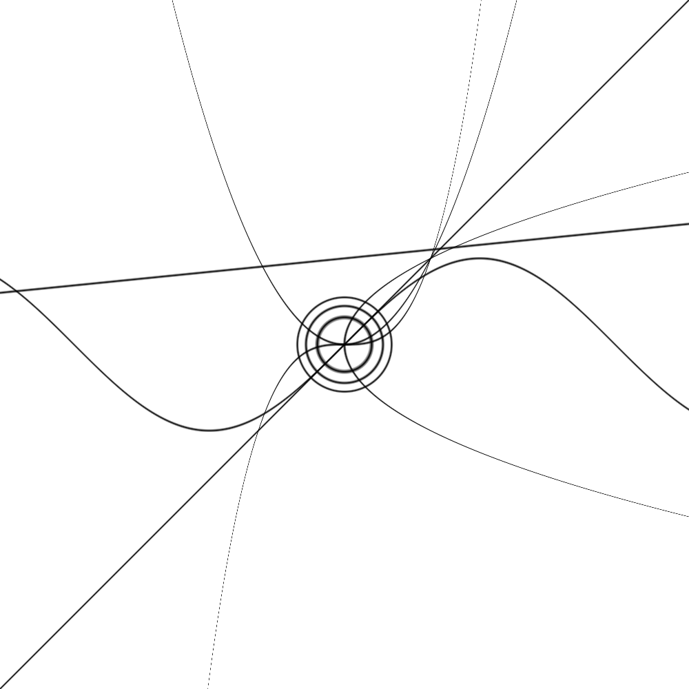
As you can see in the final image, the scaling is looking pretty good across the different functions. The function to calculate an appropriate cutoff value is shown below. Given the position we want to check, and a delta value (so that the line thickness can be changed manually), we return a cutoff value to use. The function also makes use of an accuracy value so that in cases where you would prefer faster image gen speed in exchange for less uniform lines, that can be done.

The function works for a particular function f(x, y) by calculating abs(f(x + d, y) - f(x - d, y)), for the horizontal direction, and similarly for the other directions. This gives a value for how the function changes in a small area. taking the largest change acros all directions gives a value that is bigger the larger the change is. We can then use this as a cutoff value. It isn’t a perfect solution, but it works well enough for the graphs that I have checked.

;; check how fn changes along horz, vert and diag
(flet 
 ((calc-cutoff
   (fn x y delta)
   (flet
    ((cutoff-fn
      (dx dy)
      (let ((delta  (/ delta (sqrt (+ (abs dx) (abs dy))))))
	(flet
	 ((calc (dx dy)
		(funcall fn
			 (+ x (* dx delta))
			 (+ y (* dy delta)))))
	 (abs (- (calc dx dy) (calc (* dx -1) (* dy -1))))))))
    (max (if (< accuracy 1)
	     delta 0)
	 (if (>= accuracy 1)
	     (max (cutoff-fn 1 0) (cutoff-fn 0 1)) 0)
	 (if (>= accuracy 2)
	     (max (cutoff-fn 1 1) (cutoff-fn 1 -1)) 0)))))

I also added a parameter to the graphing functions to allow the image to be inverted:

The graphing code is generalized so each type of graph goes through the same function. This function is for graphs of the form f(x, y) = g(x, y). Functions such as f(x) = y or f(x, y) = c can be written in that form, so the graph generator for these just transform the passed functions and call the single graphing function behind the scenes.

Animation

I also added a function that can help with animating these graphs. That function works by taking as an argument a function that accepts an animation progress and returns a list of graphing functions to plot for that frame. Here is an example animation of circles.

(defun gen-circle-anim (anim-progress)
  (let
      ((fns (list))
       (circle-count 10)
       (circle-size 1.45))
    (dotimes (i circle-count)
      (let*
	  ((index i) ;; to not take a closure of i in closeness fn
	   (offset
	    (+ (- (* (/ 1
			(/ circle-count
			   2))
		     circle-size
		     index)
		  circle-size)
	       (* circle-size
		  anim-progress))))
	(if (> offset 0) ;; don't show the cirles with 0 or less radius
	    (setf
	     fns
	     (cons (canim:fn=c
		    (lambda (x y)
		      (+ (expt x 2)
			 (expt y 2)))
		    (expt offset 2)
		    :thickness 4)
		   fns)))))
    fns))

(canim:make-anim
 "build/circles/"
 100 100 100
 (canim:make-pos :scale 2 :x -1 :y -1)
 (canim:make-pos :scale 2 :x -1 :y -1)		 		 		 
 :pixel-meta-fn
 (canim:graph-anim #'gen-circle-anim))

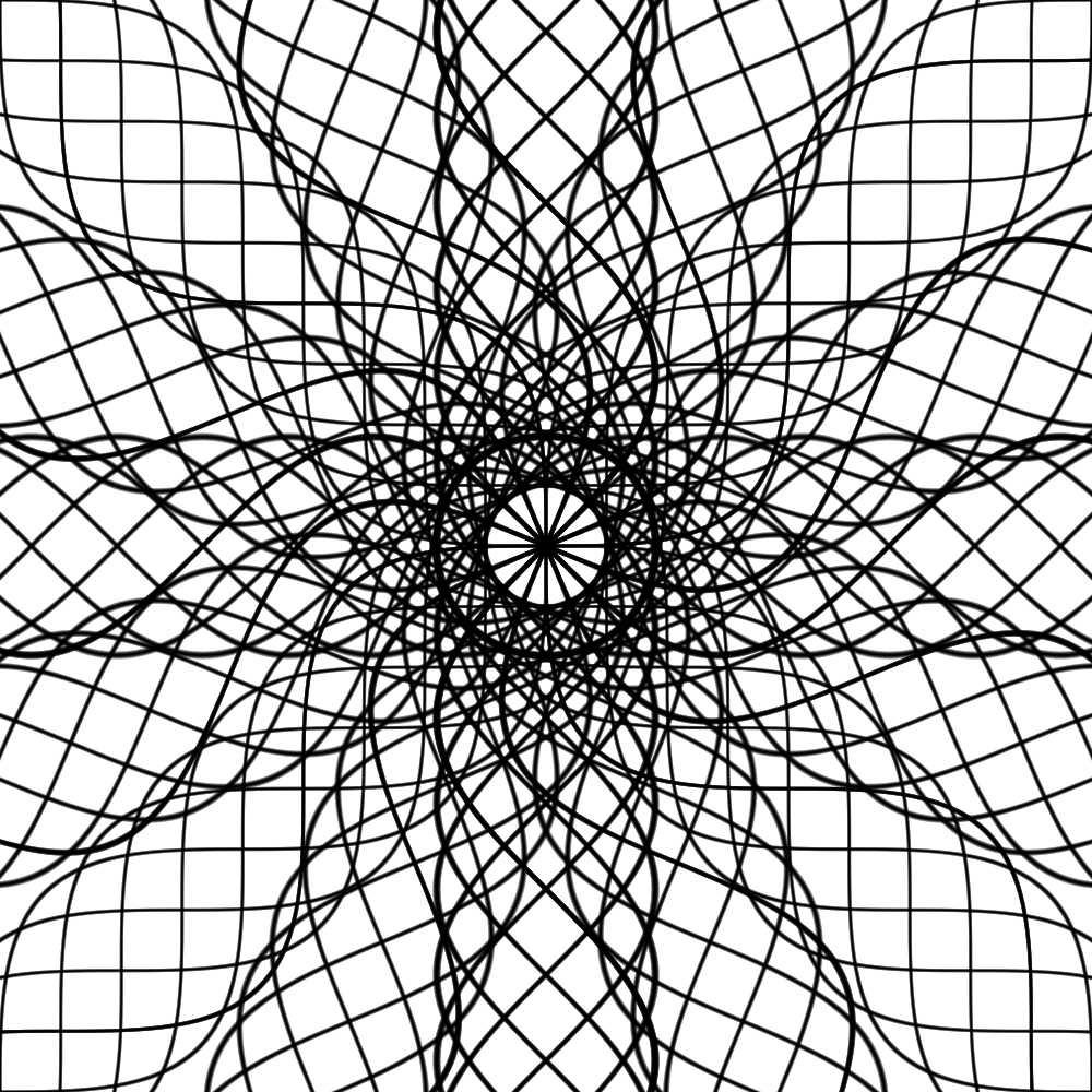
Gallery of Generated Images

The code to generate these images can be found in the demo/images folder of the source code for this project.

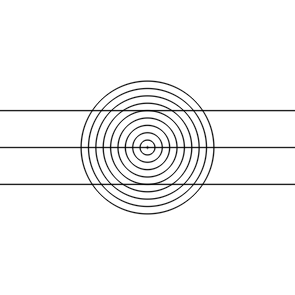
Lined Circles

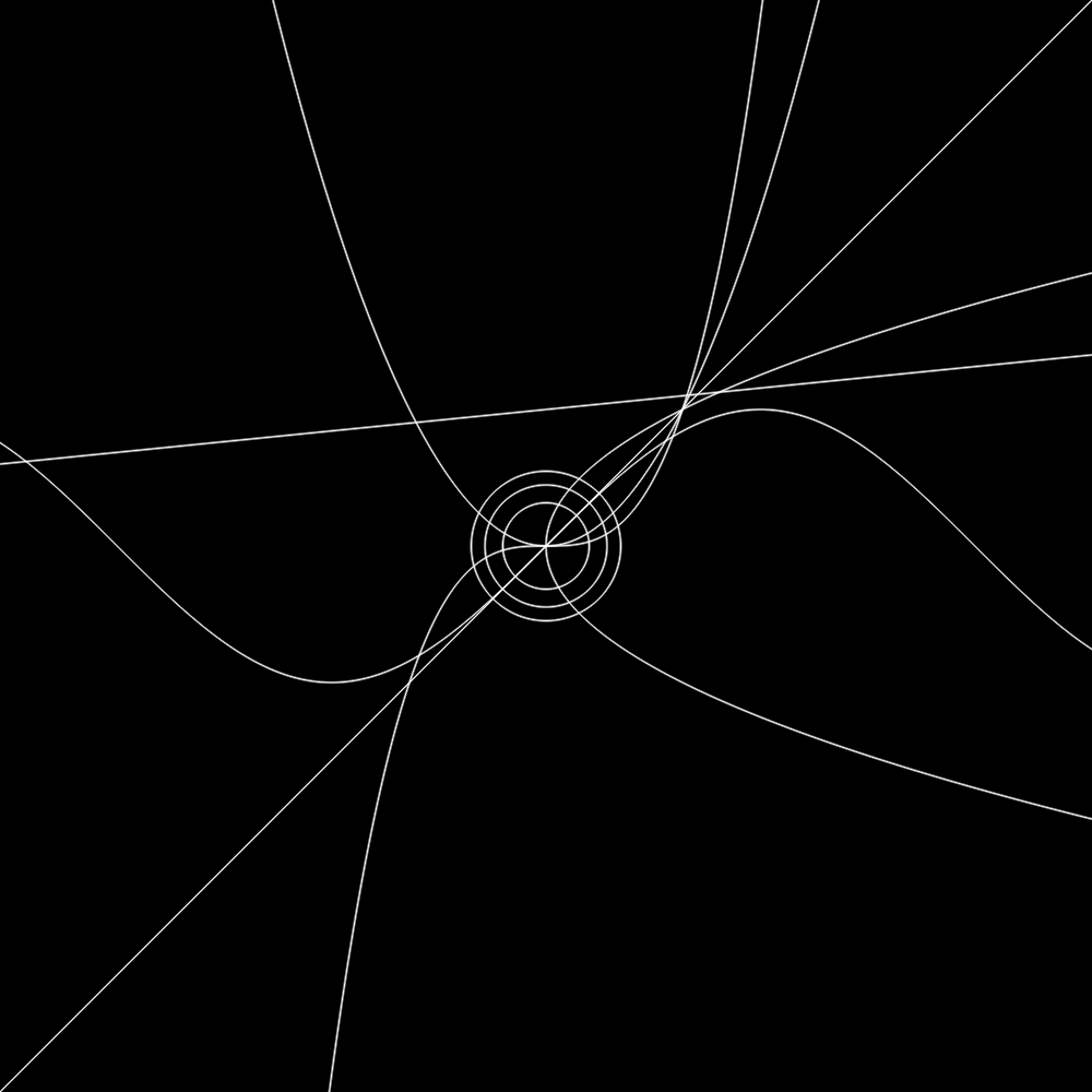
Compass

Rotated Sine

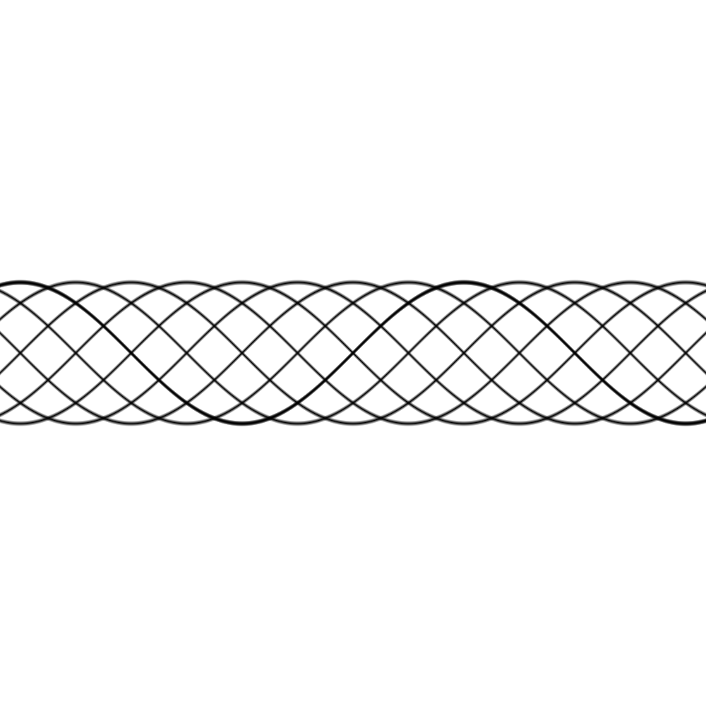
Braided Sine

Double Arch

Compass

Grid

Rotated Grid